Analyzing Linked Open Data with R
Background
The idea of statistical data analysis has never been more popular, from Nate Silver's book The Signal and the Noise: The Art and Science of Prediction to industry trends such as Big Data.
Data itself comes in a vast variety of models, formats, and sources. Users of the R language are familiar with CSV and HDF5 files, ODBC databases, and more.
Linked Data
Against this sits Linked Data, based on a graph structure: simple triple statements (entity-attribute-value or EAV) using HTTP URIs to denote and dereference entities, linking pools of data by means of shared data and vocabularies (ontologies).
For example, a photography website might use an entity for each photo it hosts, which, when dereferenced, displays a page-impression showcasing the photograph with other metadata surrounding it. This metadata is a blend of the WGS84 geo ontology (for expressing a photo's latitude and longitude) and the EXIF ontology (for expressing its ISO sensitivity). By standardizing on well-known ontologies for expressing these predicates, relationships can be built between diverse fields. For example, UK crime report data can be tied to Ordnance Survey map/gazetteer data; or a BBC service can share the same understanding of a musical genre as Last.FM by standardizing on a term from the MusicBrainz? ontology.
The lingua franca of Linked Data is RDF, to express and store the triples, and SPARQL, to query over them.
Worked Example
The challenge: to explore the United Kingdom's population density using data from DBpedia.
Collating the Data
We start by inspecting a well-known data-point, the city of Edinburgh.
The following URLs and URI patterns will come in handy:
- http://dbpedia.org/sparql - the DBpedia SPARQL endpoint against which queries are executed
- http://en.wikipedia.org/wiki/Edinburgh - a page in Wikipedia about Edinburgh
- dbpprop:title - a CURIE, identifying the title attribute within the dbpprod namespace (http://dbpedia.org/property/), thereby assigning a title ("The City of Edinburgh").
- http://dbpedia.org/resource/Edinburgh - an identifier for a DBpedia resource, comprised of data automatically extracted from the corresponding Wikipedia page; if you view it in a Web browser, it redirects to:
- http://dbpedia.org/page/Edinburgh - a human-readable view of the DBpedia resource, showing its attributes and values
On examining the last of these, we see useful properties such as
dbpedia-owl:populationTotal 495360 (xsd:integer)
This tells us that dbpedia-owl:populationTotal is a useful predicate by which to identify a settlement's population. (Note: we do not need to search for entities of some kind of "settlement" type; merely having a populationTotal implies that the entity is a settlement and choosing the wrong kind of settlement - stipulating "it has to be a town or a city" would risk losing data such as villages and hamlets.)
Looking further down the page, we see the two properties:
geo:lat   55.953056  (xsd:float)
geo:long  -3.188889  (xsd:float)
Again, we do not need to know the type of the entity; that it has a latitude and longitude is sufficient.
So far, we have some rudimentary filters we can apply to dbpedia: to make a table of latitude, longitude, and corresponding population.
Finally, we can filter it down to places in the UK, as we see the property:
dbpedia-owl:country dbpedia:United_Kingdom
Constructing the SPARQL Query
We can build a SPARQL query using the above constraints, thus:
prefix      dbpedia: <http://dbpedia.org/resource/>
prefix  dbpedia-owl: <http://dbpedia.org/ontology/>

SELECT DISTINCT  ?place
                 ?latitude
                 ?longitude
                 ?population
  WHERE
    {
      ?place          dbpedia-owl:country  <http://dbpedia.org/resource/United_Kingdom> .
      ?place  dbpedia-owl:populationTotal  ?population                                  .
      ?place                      geo:lat  ?latitude                                    .
      ?place                     geo:long  ?longitude                                   .
    }
  ORDER BY ?place
  LIMIT 100
and the resultset looks like:
| place | latitude | longitude | population |
|---|---|---|---|
| http://dbpedia.org/resource/Aberporth | 52.1333 | -4.55 | 2485 |
| http://dbpedia.org/resource/Accrington | 53.7534 | -2.36384 | 35203 |
| http://dbpedia.org/resource/Acomb,_North_Yorkshire | 53.955 | -1.126 | 22215 |
| http://dbpedia.org/resource/Adamstown,_Pitcairn_Islands | -25.0667 | -130.1 | 48 |
| http://dbpedia.org/resource/Aldeburgh | 52.15 | 1.6 | 2793 |
| http://dbpedia.org/resource/Aldershot | 51.247 | -0.7598 | 33840 |
| http://dbpedia.org/resource/Alkborough | 53.6835 | -0.667179 | 455 |
| http://dbpedia.org/resource/Alkborough | 53.6856 | -0.667179 | 455 |
| http://dbpedia.org/resource/Alkborough | 53.6835 | -0.6658 | 455 |
| http://dbpedia.org/resource/Alkborough | 53.6856 | -0.6658 | 455 |
| http://dbpedia.org/resource/Ambleside | 54.4251 | -2.9626 | 2600 |
| http://dbpedia.org/resource/Applecross | 57.433 | -5.80958 | 544 |
| http://dbpedia.org/resource/Arthington | 53.9 | -1.58 | 561 |
| http://dbpedia.org/resource/Ashington | 55.181 | -1.568 | 27335 |
Data Sanitization
However, on executing this against the DBpedia SPARQL endpoint, we see some strange "noise" points. Some of these might be erroneous (Wikipedia being human-curated), but some of them arise from political arrangements such as the remains of the British Empire ? for example, Adamstown in the Pitcairn Islands (a British Overseas Territory, way out in the Pacific Ocean). Hence, to make plotting the map easier, the data is further filtered by latitude and longitude to points within a crude rectangle surrounding all the UK mainland.
prefix      dbpedia: <http://dbpedia.org/resource/>
prefix  dbpedia-owl: <http://dbpedia.org/ontology/>

SELECT DISTINCT ?place
                ?latitude
                ?longitude
                ?population
  WHERE
    {
      ?place          dbpedia-owl:country  <http://dbpedia.org/resource/United_Kingdom> .
      ?place  dbpedia-owl:populationTotal  ?population                                  .
      ?place                      geo:lat  ?latitude                                    .
      ?place                     geo:long  ?longitude                                   .
      FILTER (      ?latitude > 50
               AND  ?latitude < 60
               AND ?longitude < 2
               AND ?longitude > -7
             )
    }
Map
The GADM database of Global Administrative Areas site has free maps of country outlines available for download as Shapefiles, ESRI, KMZ, or R native. In this case, we download a Shapefile, unpack the zip archive, and move the file GBR_adm0.shp into the working directory.
R
There is an R module for executing SPARQL queries against an endpoint. We install some dependencies as follows:
> install.packages("maptools")
> install.packages("akima")
> install.packages("SPARQL")
The maptools library allows us to load a Shapefile into an R data frame; akima provides an interpolation function; and SPARQL provides the interface for executing queries.
The Script
#!/usr/bin/env Rscript

library("maptools")
library("akima")
library("SPARQL")

query<-"prefix      dbpedia: <http://dbpedia.org/resource/>
prefix  dbpedia-owl: <http://dbpedia.org/ontology/>

SELECT DISTINCT ?place
                ?latitude
                ?longitude
                ?population
  WHERE
    {
      ?place          dbpedia-owl:country  <http://dbpedia.org/resource/United_Kingdom> .
      ?place  dbpedia-owl:populationTotal  ?population                                  .
      ?place                      geo:lat  ?latitude                                    .
      ?place                     geo:long  ?longitude                                   .
      FILTER (      ?latitude > 50
               AND  ?latitude < 60
               AND ?longitude < 2
               AND ?longitude > -7
             )
    }"

plotmap<-function(map, pops, im) {
  image(im, col=terrain.colors(50))
  points(pops$results$longitude, pops$results$latitude, cex=0.25, col="#ff30000a")
  contour(im, add=TRUE, col="brown")
  lines(map, xlim=c(-8,3), ylim=c(54,56), col="black")
}

q100<-paste(query, " limit 100")

map<-readShapeLines("GBR_adm0.shp")

if(!(exists("pops"))) {
  pops<-SPARQL("http://dbpedia.org/sparql/", query=query)
}

data <- pops$results[with(pops$results, order(longitude,latitude)), ]
data <- data[with(data, order(latitude,longitude)), ]
im <- with(data, interp(longitude, latitude, population**.25, duplicate="mean"), xo=seq(-7,1.25, length=200), yo=seq(50,58,200), linear=FALSE)

plotmap(map, pops, im)

fit<-lm(population ~ latitude*longitude, data)
print(summary(fit))

subd<-data[c("latitude","longitude","population")]
print(cor(subd))
Run this interactively from R:
bash$ R
...
> source("dbpedia-uk-map.R")
...
After a few seconds to load and execute the query, you should see a map showing the outline of the UK (including a bit of Northern Ireland) with green/yellow heat-map and contour lines of the population density. Individual data-points are plotted using small blue dots.
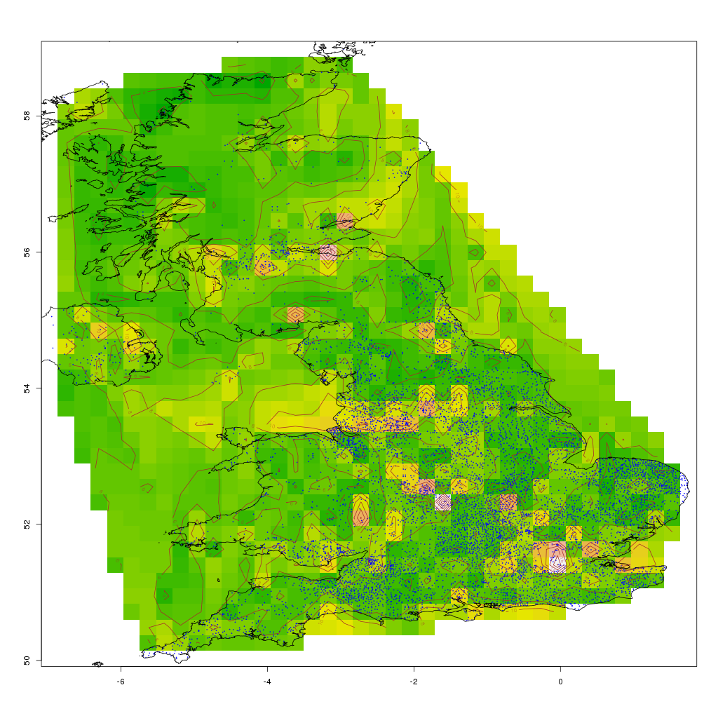
This is a rather na?ve plot: interpolation is not aware of water, so interpolates between Stranraer and Belfast regardless of the Irish Sea in the way; however, it looks reasonable on land, with higher values over large centers of population such as London, the Midlands, and the central belt in Scotland (from Edinburgh to Stirling to Glasgow).
The script runs two statistical analyses:
- a simple linear regression of population with latitude and longitude:
Call:
lm(formula = population ~ latitude * longitude, data = data)

Residuals:
     Min       1Q   Median       3Q      Max
  -37155   -17695   -12856    -8212 62278176

Coefficients:
                    Estimate   Std. Error   t value   Pr(>|t|)
(Intercept)        -273340.2     478917.6    -0.571      0.568
latitude              5489.0       9139.8     0.601      0.548
longitude           -41694.5     146956.3    -0.284      0.777
latitude:longitude     776.8       2788.6     0.279      0.781

Residual standard error: 660500 on 9206 degrees of freedom
Multiple R-squared: 7.733e-05,  Adjusted R-squared: -0.0002485
F-statistic: 0.2373 on 3 and 9206 DF,  p-value: 0.8704
- correlation between latitude, longitude and population, shown as a matrix:
                 latitude      longitude    population
latitude      1.000000000   -0.291285847   0.008083111
longitude    -0.291285847    1.000000000  -0.004161835
population    0.008083111   -0.004161835   1.000000000
This shows a very slight correlation of population-density with longitude, and about twice as much correlation with latitude, but neither is statistically significant in the given data (as the p value should be less than 0.01, not up around 0.5-0.8).
Next Steps
SPARQL has a SERVICE keyword that allows federation, i.e., the execution of queries against multiple SPARQL endpoints, joining disparate data by common variables (a/k/a SPARQL-FED). For example, it should be possible to enrich the data by blending Geonames and the Ordnance Survey gazetteer in the query.
Over to you to explore the data some more!